This post is dedicated to my idea of building an end-to-end machine learning project, walking you through the major steps involved in developing a working Machine Learning solution, albeit I will not be covering packaging and deploying the solution in this post. That will be coming up shortly, this part focuses on building a model for to solve a business need.

#Major steps covered in a machine learning project are:

• Understanding and framing the problem

• Getting the data

• Explore the data

• Prepare the data

• Apply the algorithms to create models

• Fine-tune the models to reduce errors

• Present the solutions

• Deploy the ML system

Lets get started...

###STEP 1: Frame The Problem This is essentially the first step in any machine learning project. Before a viable solution can be achieved, the right questions must be asked to understand what challenges the project is meant to overcome,and what type of machine learning solution is to be applied. This phase highlights understanding of how machine learning can be applied as a solution to the needs of the business. So, our project in this article will be predicting the concrete compressive strength for a client, based on sensor-collected data from factory machines, and giving insight on what factors have the most effect on the concrete compressive strength. This is a regression problem,and supervised machine learning will be better employed.

###STEP 2: Getting the data: Machine learning is heavily reliant on data, so every machine learning project must inquire on questions such as: What type of data is needed? How can the data be sourced? How available is the data? What are the legal requirements for such data?. When all these questions have been provided for and there is available data, the data is loaded to a virtual environment and converted to a format it can be worked on. Necessary libraries are imported, and then the engineering part of the project can begin.

###STEP 3: Load the data set

• Launch a virtual environment for the project and open the terminal. This could be on your local machine using the Anaconda Navigator, but I would recommend using Google's free online machine via Google Colab.

• Import the necessary libraries

• Next will be to load the data set and assign it to a variable called "data".

data = pd.read_excel('http://archive.ics.uci.edu/ml/machine-learning-databases/concrete/compressive/Concrete_Data.xls')

###STEP 4: Explore the data The next thing to do is to investigate the data to gain some insight into what properties the data contains. This phase usually involves domain knowledge of the subject matter, as human experts may be sought to better aid the developer understand some key assumptions to be made on the data, and gain useful insight.

• Nature of the data set: Find out how many rows and columns our dataset has, and check for the data types contained within the dataset using the .info() method.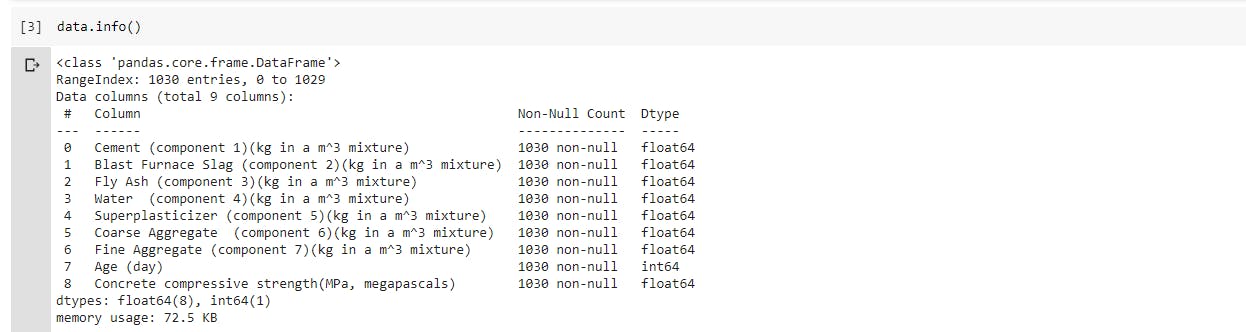 So it happens to be that we have a total of 9 columns and 1030 rows, with no categorical features/columns in the dataset (i.e the entire dataset is made of numerical values) the data is also not having any missing values, so we are indeed gaining some insight into how well suitable the data is for the estimators that will be used later on.

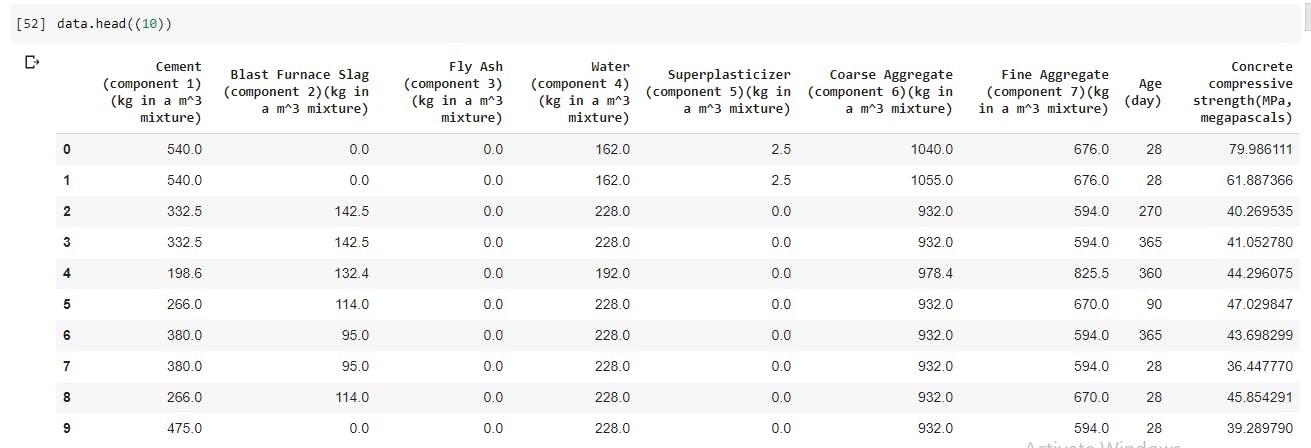
• Lets see the first 10 rows of the dataset data.head(10)

• Find out the statistical summary of the data including the mean,count,the min and max values,and standard deviation. data.describe()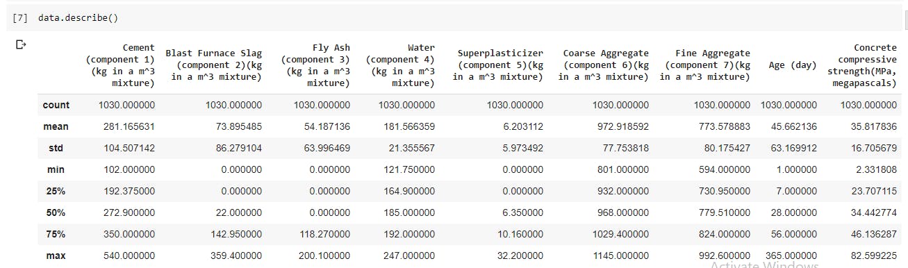

###STEP 5: Prepare the data Otherwise called data pre-processing/cleaning is essential to produce well performing models. In this stage,categorical features if present should be transformed; missing values would be addressed; features are added/selected,scaled,standardized/regularized. In some machine learning projects such as Image classification, input features may be resized and data augmented. All of these are implemented to either boost the performance of the models, or enable these models to generalize better or possibly do both.

Data augmentation is a strategy of generating more data from existing training samples without actually collecting new data, by applying random transformations that produce similar to real-life data. This exposes a model to more aspects of the data which allows it to generalize better

• The first preprocessing I'll be doing is to check for correlated features,by analyzing the correlation of each variable with the target variable. Correlated features bring the same information to the model,so it really doesn't help the model in any way. Therefore, it is logical to remove one of two highly correlated features. data.corr()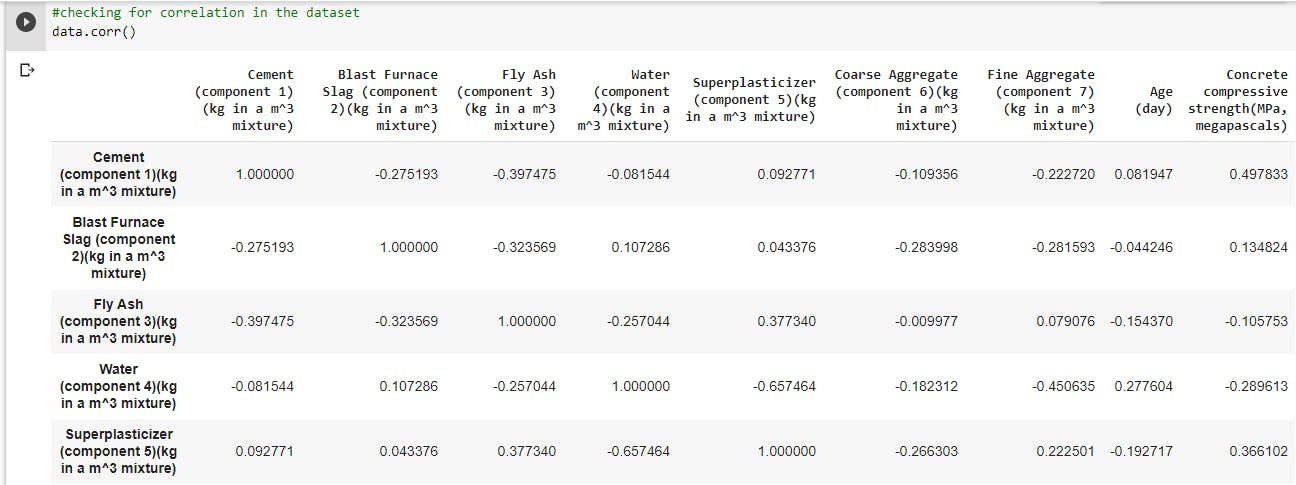 The features do not seem to have high correlation between them, so we can do without dropping any features.
• Inspect the distribution of the features: This helps to engineer understand what kind of features are being dealt with. Inspecting the distribution of the dataset also helps to identify outliers or other erroneous data in the dataset. Data can be cleaned further to help the model generalize better or improve performance. Visualize the distribution on a plot. 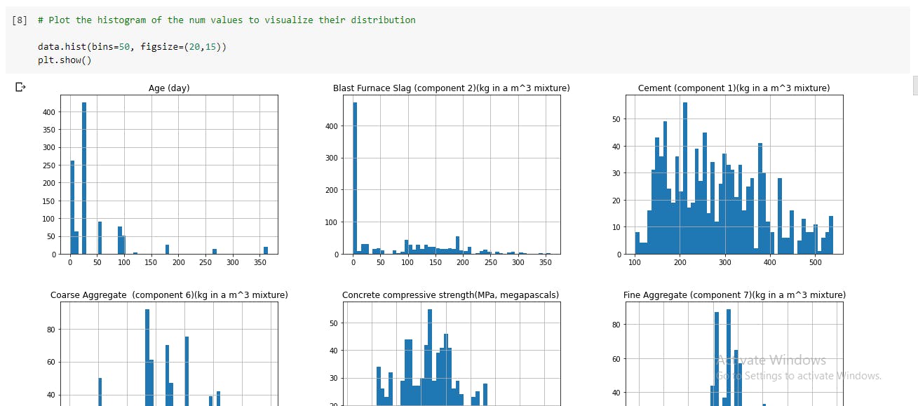The Seaborn library is also very useful here, for a much better visual display of the plot. sns.distplot(data['Cement (component 1)(kg in a m^3 mixture)'],hist=True, kde=True, bins=20) plt.show(). Boxplots can also be used to supplement the distribution plots; they are popular visual aids for spotting outliers. fig, ax = plt.subplots(figsize=(20,10)) sns.boxplot(data=data, ax=ax, orient='h');

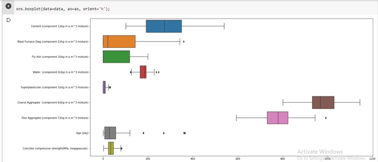Understanding the nature of outliers in the dataset is important as it affects the choice of using either standardizing or normalizing technique to regularize the data features.

###STEP 6: Building Models With the data cleaned up, algorithms can be plugged in,and used to build and train models. Different models should be built and compared to each other, the errors and assumptions made by the various model should be investigated. Considerations have to be made,regarding how to build the models(e.g building from scratch vs leveraging transfer learning).The data should also be split into training,testing and validation sets.

####Split the data into training and testing sets

from sklearn.model_selection import train_test_split
X = data.drop('Concrete compressive strength(MPa, megapascals) ', axis=1)
y = data['Concrete compressive strength(MPa, megapascals) ']
X_train, X_test, y_train, y_test = train_test_split(X, y, test_size=0.3, random_state=30)

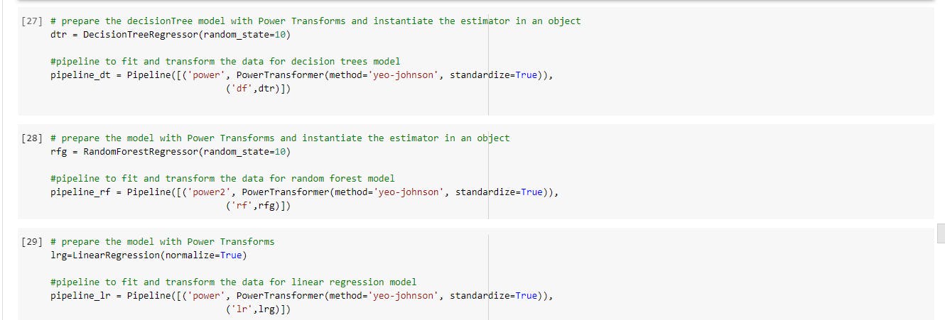
####Fitting the data with estimators I'll be using the sklearn's pipeline module to carry out some transformations, and build some models. I'll be using the Linear Regression, Decision Trees Regressor estimator,and the Random Forest regressor estimator to build models, and compare them.

 from sklearn.pipeline import Pipeline
 from sklearn.preprocessing import PowerTransformer
 from sklearn.metrics import r2_score
 from sklearn.metrics import mean_squared_error as mse
 from sklearn.tree import DecisionTreeRegressor
 from sklearn.linear_model import LinearRegression
 from sklearn.ensemble import RandomForestRegressor
 from sklearn.ensemble import AdaBoostRegressor

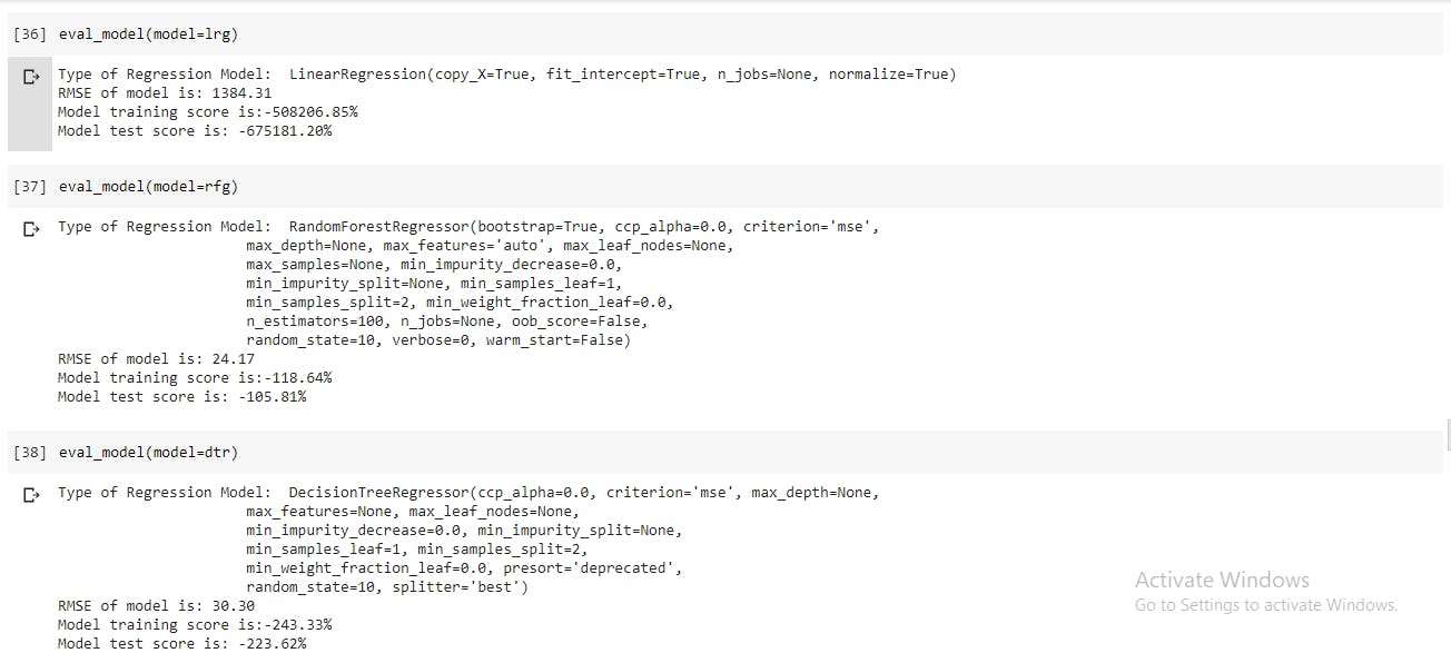
• Define a function that makes prediction using a specified model and assesses the performance of the model printing the model evaluation score: root_mean_squared_error, training score and r2_score

# Function to evaluate and print model performance
def eval_model(model):
    """
    This function will make predictions for the specified model
    and print the model evaluaytion score: root_mean_squared_error, training score and r2_score

    Parameters:
    model: the model to use for prediction and to be evaluated

    """
    # Make prediction
    y_pred = model.predict(X_test)

    # calculate rmse
    rmse = np.sqrt(mse(y_test, y_pred))

    # Calculate model training performnace
    model_score = model.score(X_train, y_train)

    # Calculate model r2_score
    r2_Score = r2_score(y_test, y_pred)

    # Print the scores
    print('Type of Regression Model: ', model)

    print("RMSE of model is: {:.2f}".format(rmse))

    print("Model training score is:{:.2f}%".format(model_score*100))

    print("Model test score is: {:.2f}%".format(r2_Score*100))
    return

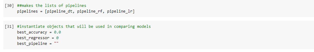
• The use of pipelines makes fitting and training the models with the various estimators quite simple, and time efficient. These estimators are used with their default hyper-parameters, so lets compare across the three which is performs better at default. 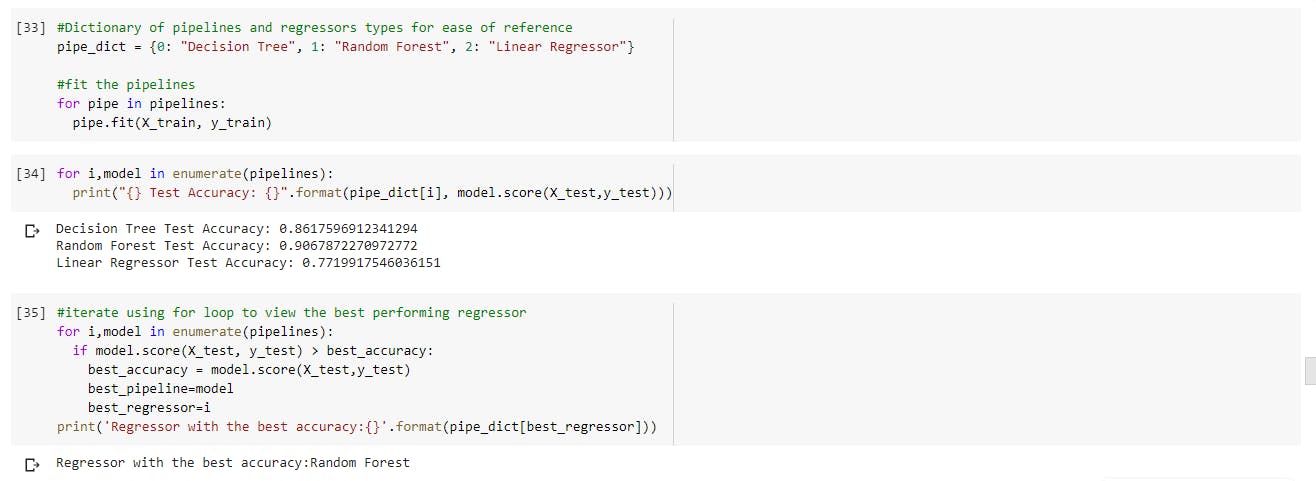The best model seems to be coming from the random forest estimator, lets view the various RMSE scores of the models. I'll be focusing on tree-based estimators in the remaining part of this post.

###STEP 6: Fine Tuning The Models(Hyper-parameter tuning): After building and training models, we can further optimize their performance by tuning their hyper-parameters. Models are kind-of like radio stations with frequencies,and knobs to fine tune the dial for enhanced audio. For model tuning,it can be done manually by repeatedly trying various tunes for different hyper-parameters of the model; or it can be done automatically using modules like GridSearchCV or RandomSearchCV.

#Import GridSearchCV
from sklearn.model_selection import GridSearchCV

#create objects to instantiate estimators
rfg2=RandomForestRegressor(random_state=40)
dtr2=DecisionTreeRegressor(random_state=40)
ada1=AdaBoostRegressor(base_estimator= DecisionTreeRegressor(random_state=40))
ada2=AdaBoostRegressor(base_estimator= LinearRegression(normalize=True))

#create a pipeline
pipe = Pipeline([("Regrezzor", RandomForestRegressor())])

#create dictionary with candidate learning algorithms and their hyperparameters
grid_param = [
             {"Regrezzor": [rfg2],
              "Regrezzor__n_estimators" : [5,11,18,25],
              "Regrezzor__max_features": ["auto", "sqrt", "log2"],
              "Regrezzor__min_samples_split": [2,4,6,8],
              "Regrezzor__oob_score": [True, False],
              "Regrezzor__max_depth": [range(1,10), None],
              "Regrezzor__bootstrap": [True, False]},

              {"Regrezzor": [dtr2],
              "Regrezzor__max_depth": range(1,10),
              "Regrezzor__splitter": ['best', 'random'],
              "Regrezzor__min_samples_split": [2,4,6,8],
              "Regrezzor__max_leaf_nodes": [None, range(1,5)]},

              {"Regrezzor": [ada1],
              "Regrezzor__base_estimator__max_depth": range(1,10),
              "Regrezzor__n_estimators":[50,100,200],
              "Regrezzor__learning_rate":[0.15,0.3,0.45,0.66,0.75,1.0]
               },

              {"Regrezzor": [ada2],
              "Regrezzor__n_estimators":[50,100,200],
              "Regrezzor__learning_rate":[0.15,0.3,0.45,0.66,0.75,1.0]
               }              
]

#fit gridsearch on the pipelines and select the best model
gridSearch = GridSearchCV(pipe, grid_param, cv=5, verbose=0, n_jobs=-1)
best_model = gridSearch.fit(X_train, y_train)
print(best_model.best_estimator_)
print("The mean accuracy of the model is:",best_model.score(X_test,y_test))

So, in the above cell I'm comparing four models via three(3) ensemble methods, to derive the best model. GridSearch will run through all of them, and store the best model in the "best_model" object. Automating the hyper-parameter tuning is always the recommended option, as its easier to replicate results and provide consistency than when manual tuning is employed.

-Assess the model by calling the evaluation function eval_model(best_model). The result is displayed below:

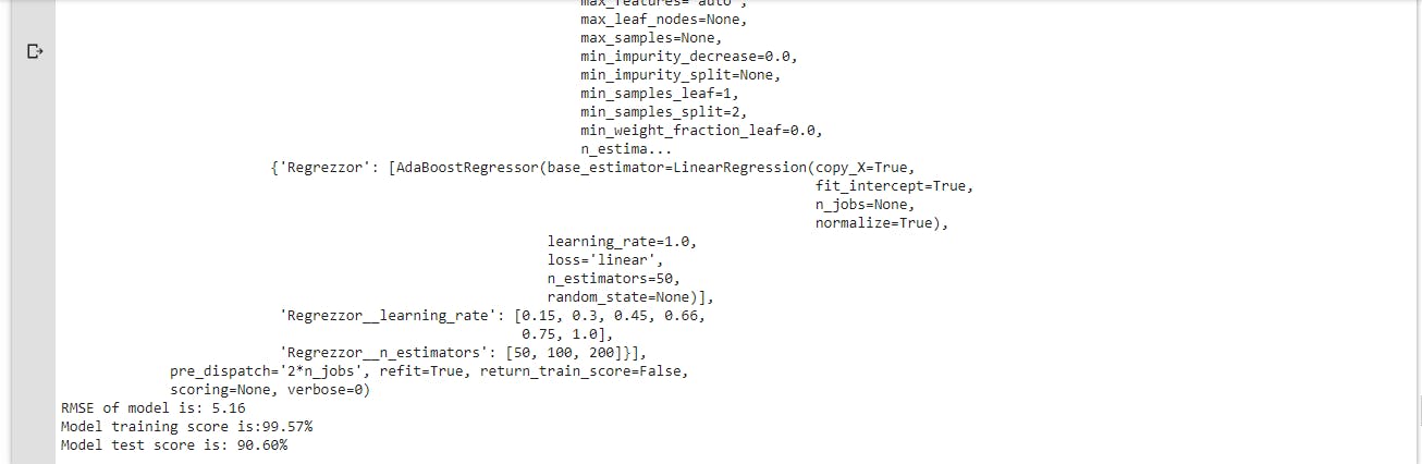
• The result gotten after automated hyper-parameter tuning produced the best result with the least errors compared to previous models with default estimators, its shows just how important tuning the models of an ML project can be.

###STEP 7: Presenting the Solution: After building,training and selecting the best model to meet the business/client's needs; the business solution has to be presented to relevant stakeholders. This is a much less technical aspect of the project but it requires effective communication and data visualization skills. This stage of the project is intent on infusing confidence into the client, and prove the that the solution proposed meets the objective.

###STEP 8: Deploy the ML Solution: The machine learning system has to be made ready for production,it may be plugged into an already existing wider system or strategy.As a software solution, It should be exposed to unit testing prior,and adequately monitored once up and running. Models will have to be retrained or updated to combat data drift,and this process must be considered and catered to.

##Summary After experimenting with some other models, I was able to produce a better model that performed well on my dataset, I was also able to investigate my model, to see what features were having more impact on my target feature, by using permutation feature importance to determine which features were more relevant. You have also discovered step-by-step how a machine learning project can be implemented end-to-end. Please leave a comment, if you have any feedback or suggestions. Bravo, Until next time....